What Is A Kalman Filter

The Kalman Filter: An algorithm for making sense of fused sensor insight

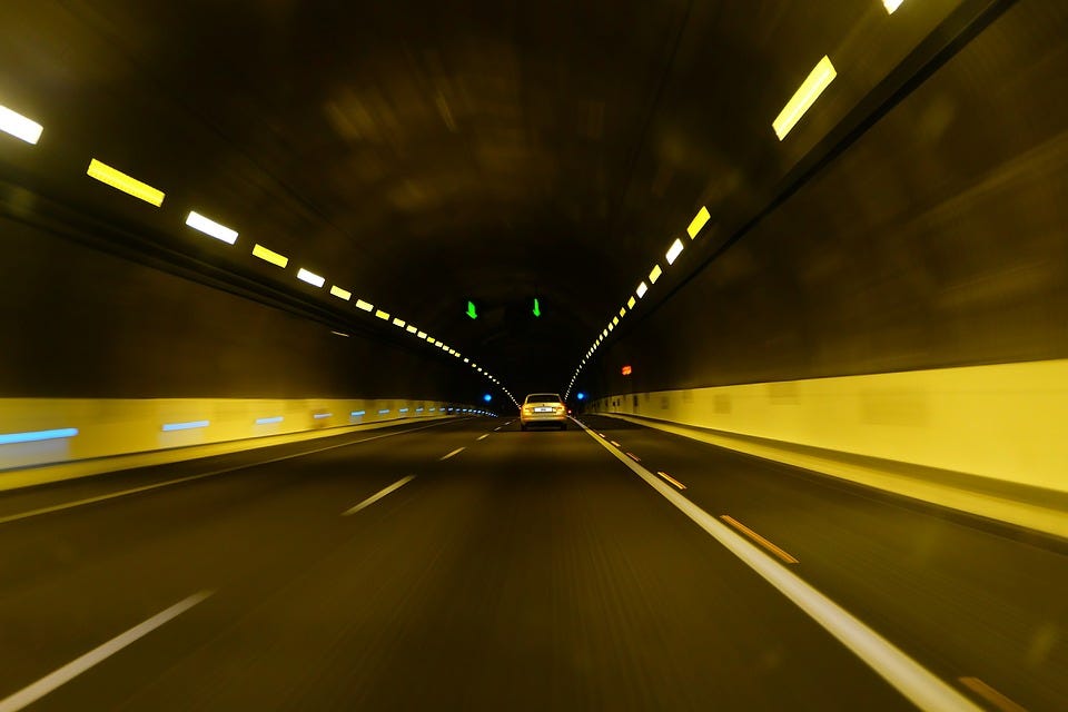
You lot're driving your motorcar through a tunnel. The GPS signal is gone. Still, you might desire to become notified that you lot should take the exit in the tunnel. How should we navigate on a auto inside a tunnel, which should know where it is right at present given only the last position?

A Short Note on Sensors

Global Positioning System receivers calculate their locations by analyzing signals that they receive from satellites. These signals don't pass through solid objects. A GPS in a vehicle may have an external antenna, or it may option upwardly plenty of bounced bespeak out of the air to operate. If signals in a tunnel are as well weak, the GPS may withal role, depending on its quality and features.

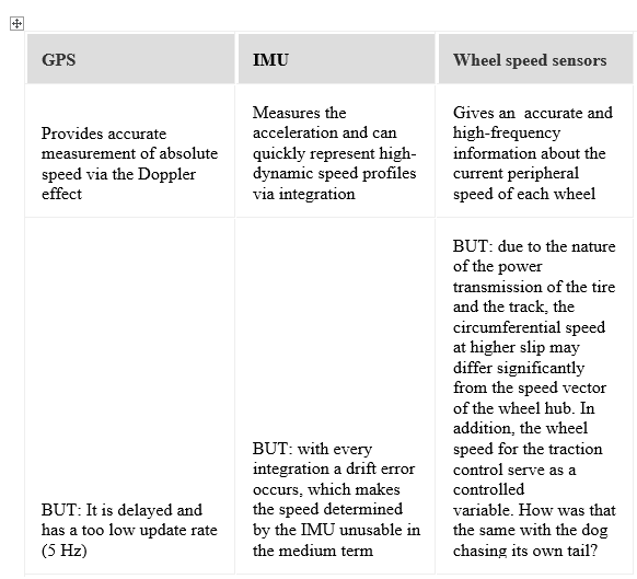
The table explains the pros and cons of each some of the sensors.

An approach that merges the vehicle sensors, tin can calculate the position .

The Measurement from the sensors

Assume that we were at the tunnel entrance and we were driving at 50km / h, and then the navigation can indeed be calculated exactly where (x = position) we would exist one minute (t = time) after.

Both the sensors take random errors, the transmission path has interference, and the resolution of CAN bus or analog-to-digital converters can cause many inaccuracies in the simple statement "speed".

For example, a speed signal looks like this:

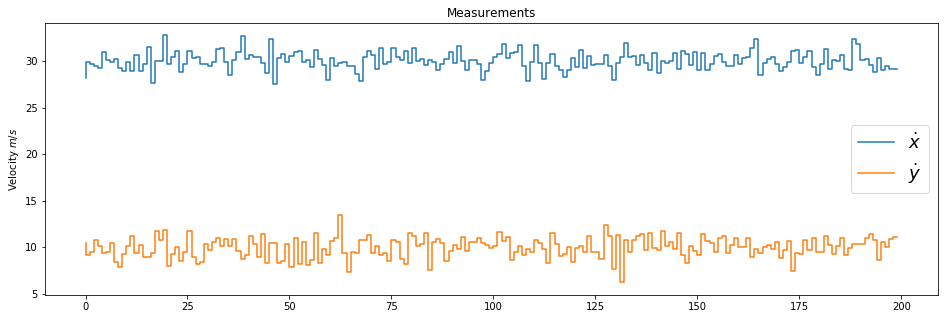
The Velocity is considered to be with a variance on both the axes. (image source)

On average, the measured speed has some "noise" added to it which differentiates them from the basis truth. If one calculates a histogram of the determined speeds, one sees that the adamant values are approximately subject to a normal distribution.

Then in that location is ane, and really but one, maximum value (unimodal) and a spread (variance). If this is the case, nosotros can do the calculation very well with a trick nevertheless.

Idea of the Kalman filter in a unmarried dimension

I would like to beginning explain the idea of the Kalman filter (according to Rudolf Emil Kalman ) with only 1 dimension . The following explanation is borrowed from the Udacity CS373 grade by Prof. Sebastian Thrun.

Calculated noise helps

In order to perform the calculation optimally despite measurement racket, the "how strong" parameter must exist known. This "how strong" is expressed with the variance of the normal distribution. This is adamant in one case for a sensor that is being used and and so uses but this "uncertainty" for the calculation.

In the following, information technology is no longer calculated with accented values but with mean values (μ) and variances σ ² of the normal distribution. The mean of the normal distribution is the value that we would want to calculate. The variance indicates how conviction level. The narrower the normal distribution (depression variance), the confident the sensors are with the measurements.

A sensor that measures 100% exactly has a variance of σ ²= 0 (information technology does not exist).

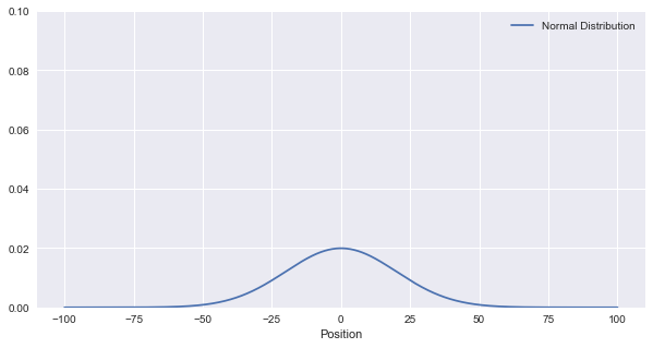
Allow'due south assume that the GPS signal has just been lost and the navigation organisation is completely unclear where you are. The variance is high, the curve corresponding is actually flat. There is an uncertainty.

Normal distribution with variance = 20 and mean = 0

The Uncertainty is High, as the variance is in a large magnitude.(paradigm-source)

Now comes a speed measurement from the sensor, which is also "inaccurate" with advisable variance. These two uncertainties must now exist linked together. With the assistance of Bayes rule, the add-on of two Gaussian function is performed . Prof. Thrun explains this very clearly in the Udacity CS373 course.

The two pieces of information (one for the current position and i for the measurement incertitude of the sensor) actually gives a better effect!. The narrower the normal distribution, the confident the event. Movement worsens the estimate.

Of course, the vehicle as well moves, which adversely affects the accuracy of the position conclusion. A sensor, for example, can make up one's mind the rotation of the cycle and make the assumption of the radius of the cycle and could take a decision on the altitude traveled, just this volition always remain somewhat inaccurate. This inaccuracy of movement is as well described with a normal distribution. Computing with the electric current judge runs a niggling differently this time, because the "movement" can likewise be chosen "Prediction". You tin estimate after the calculation, where you volition exist next (measurement) time.

In our example, μ is simply v * dt, which is the distance we had traveled in the calculation fourth dimension.

A simple implementation of this is:

          def predict(mean1, var1, mean2, var2):
            new_mean = mean1 +mean2
            new_var = var1 + var2
            return [new_mean, new_var]

Measuring & Updating: The Kalman filter

The Kalman filter but calculates these two functions over and once again.

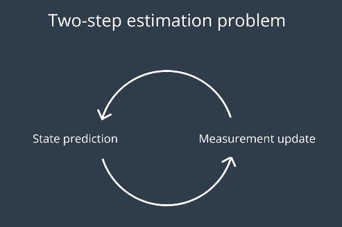
The filter cyclically overrides the hateful and the variance of the result. The filter will always be confident on where it is, equally long as the readings do not deviate too much from the predicted value.

A new measurement improves the guess

Since the measured values (in update) fit relatively well to the predicted ones (by predict), the filter improves footstep by pace to ensure that it is correct (normal distributions become narrower and higher), even though the values are noisy.

          def update(mean1, var1, mean2, var2):               sum = var1+var2
              pr_s = mean1*var2 + mean2*var1
              #impress(pr_s)
              new_mean =1/(sum) * pr_s
              production = var1*var2
              new_var = product/sum
              return [new_mean, new_var]

Without matrices, you lot can merely count in one dimension, which is bereft for…

Multidimensional Kalman filter

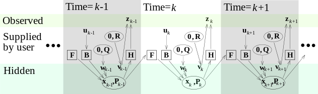
The Picture Illustrates the Kalman Filter 'southward Predition footstep in various time-stages. (Epitome Source)

I would similar to explain the procedure once again using the example of a vehicle with navigation device, which enters a tunnel. The final known position is before losing the GPS point. Afterwards only the speed information of the vehicle (wheel speeds & yaw charge per unit) is available as a normal distributed noisy measured variable. From here, the velocity is calculated.

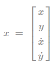
Nosotros now turn to the more complicated part. The procedure mentioned with multiplying or calculation the mean values and variances thus only works in the one-dimensional case. In the multi-dimensional problem, we would take the mean and the variance inside a matrix on which all the operations are performed.That is, when the state you want to mensurate can exist fully described with just one variable. The example, which was mentioned at the beginning, to determine the position of a vehicle in the tunnel, can no longer be completely described with a variable. Although merely interested in the position, just this is already a two dimensional problem in the aeroplane. In addition, but the velocity can be measured, not the position directly. This results in a Kalman filter with the following state variables.

The state matrix consists of position and velocity in the x and y coordinates.

Initial conditions / initialization

System state X

At the beginning we will take to initialize with an initial state. In the ane dimensional instance the land was a vector.

If goose egg is known, you can simply enter zero here. If some boundary atmospheric condition are already known, they tin be communicated to the filter. The choice of the following covariance matrix controls how fast the filter converges to the right (measured) values

Co-variance matrix P

An uncertainty must be given for the initial state . In the one-dimensional instance, the variance was a vector, but now is matrix of uncertainty for all states. Here is an example with for all the four states.

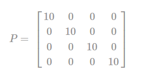
The covariance matrix consists of dubiety in the position and the velocity in the ten and y coordinates.

This matrix is well-nigh likely to be changed during the filter passes. It is changed in both the predict and right steps. The Matrices can be initialized on the basis of the sensor accuracy. If the sensor is very accurate, small values should be used hither. If the sensor is relatively inaccurate, large values should exist used here to allow the filter to converge relatively quickly. If the sensor is very accurate, modest values should be used here.

Dynamics matrix A

The core of the filter, nevertheless, is the following definition, which we should fix with great understanding of the physical context. This is not easy for many real problems. For our elementary example (in-plane movement), the physics backside information technology comes from the polish motion. For the state matrix shown above, the dynamics in matrix note is every bit follows:

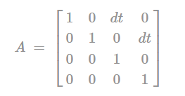
The Dynamic matrix helps us in defining the equations for predicting the Vehicle Motility Model.

This states "where" the state vector moves from 1 calculation footstep to the next within. This dynamic model is in our example is "constant velocity" model because it assumes that the velocity remains constant during a filter's adding step(dt).

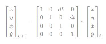
This is the prediction footstep for the State matrix.

This but reflects concrete relationships for the compatible motion. A higher form would exist the Constant Acceleration model, which would be a 6-D filter and still includes the accelerations in the land vector. In principle, other dynamics can be specified here.

Process noise co-variance matrix Q

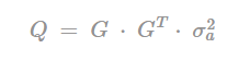
As the movement of the vehicle (in the sense of a superimposed, commonly distributed racket) may also be disturbed, this is where the process noise co-variance matrix is introduced. This matrix tells united states of america about the filter , and how the system state can "bound" from one pace to the side by side. Imagine the vehicle that drives autonomously. It can exist disturbed by a gust of wind or road bumps, which has a force effect. A speed change by the commuter is besides an acceleration that acts on the vehicle. If an acceleration now affects the system land , and then the physical dependence for it is Q. The matrix is a co-variance matrix containing the following elements:

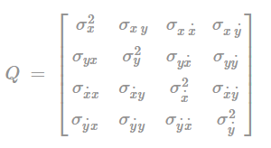
The Process Noise Co-variance matrix consist of the errors caused in the process.

It is easy to summate by placing the vector then multiplying it by the assumed standard deviation for the acceleration.

The Equations to prepare the Q matrix appropriately.

Control Matrix B and Command Input u

An external control variables (eg: steering, braking, acceleration, etc.) is possible via the control matrix . The u matrix will contain the robotic input of the system which could exist the instantaneous acceleration or the altitude traveled past the organisation from a IMU or a odometer sensor.

Measuring matrix H

The filter must also be told what is measured and how information technology relates to the land vector. In the example of the vehicle, the machine enters a tunnel with only position measured at first point, only the speed is measured! The values can be measured directly with the cistron 1.0 (ie the velocity is measured directly in the correct unit of measurement), which is why in only i.0 is set to the appropriate position.

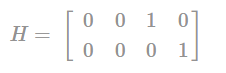
If the sensors measure in a different unit or the size by detours, the relationships in the measuring matrix must exist mapped in a formula.

Measurement noise covariance matrix R

Equally in the 1-dimensional example the variance, a measurement uncertainty must also be stated here.

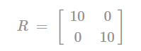
This measurement uncertainty indicates how much one trusts the measured values of the sensors. Since we mensurate the position and the velocity , this is a 2 × two matrix. If the sensor is very authentic, minor values should exist used here. If the sensor is relatively inaccurate, large values should be used here.

Unit matrix I

Last just not least, a unit of measurement matrix is necessary, which would be used to simplify the Kalman equations.

Filtering step Prediction / Predict

This office of the Kalman filter now dares to predict the state of the arrangement in the future. In improver, under certain conditions, a state tin be calculated with it which cannot be measured! That's amazing, but in our case exactly what we need. Nosotros cannot measure out the position of the vehicle considering the GPS of the navigation device has no reception in a tunnel. By initializing the state vector with a position and measuring the velocity, still, the dynamics yet be used to brand an optimal prediction about the position.

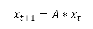
The co-variance must also be recalculated. Uncertainty almost the land of the system increases in the predict footstep, as we have seen in the 1 dimension instance. In the multidimensional case, the measurement doubtfulness is added, then the uncertainty becomes larger and larger.

P=A⋅P⋅A'+Q

That's it. The Kalman filter has fabricated a prediction statement about the expected arrangement state in the time to come or in the upcoming time-stride. The filter volition at present be measuring / correcting and checking whether the prediction of the organization state fits well with the new measurements.

The co-variance chosen to be smaller by the filter illustrates the certainty, if not, then something is wrong, which makes the filter more than uncertain.

Filter step Measure / Correct

Note : The following mathematical calculations practise not need to be derived.

From the sensors come electric current measured values, with which an innovation factor (y) is obtained by using the measurements ,the state vector with the measuring matrix .

y=Z−(H⋅x)

So it is looks at with which variance tin can be farther calculated. For this, the dubiety and the measurement matrix and the measurement doubt required.

Southward=(H⋅P⋅H′+R)

This determines the so-called Kalman gain. It states whether the readings or organisation dynamics should exist more familiar.

K= P⋅ H'S

The Kalman Gain will decrease if the readings (measurements) match the predicted organisation country. If the measured values say otherwise, the elements of matrix K become larger.

This data is now used to update the system state.

x = ten + ( K⋅ y )

And besides adamant a new co-variance for the upcoming predict step.

P= P- ( K⋅ H.P)

which is ,

P= ( I- ( Thou⋅ H) ) ⋅ P

Now it's back to the step prediction. Graphically it looks like this:

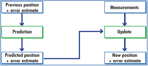
The Kalman filter could be understood as a loop (image source)

This filter runs permanently as long as measured values come in. It can likewise be open up loop, then merely the prediction footstep will be executed if no measurements are bachelor. Then the uncertainty gets bigger and bigger.

The filter at work

When we bulldoze into a tunnel , the last known position is recorded which is received from the GPS. The Kalman filter tin nevertheless predict the position of the vehicle, although it is non being measured at all time.

Now bold the vehicle speed is available nigh every twenty k/s via the Tin can double-decker, 6 iterations are merely 0.i south. The filter converges relatively apace, depending on the choice of initial weather. For example, later 100 iterations (equivalent to 2s on the vehicle), the variance is already very low, and then the filter is confident on its estimated and updates states. My implementation of the linear Kalman filter could exist plant here . The results are :

Python implementation of the Kalman filter

          def Kalman_Filter() :
            for n in range(measurements):
            x = A*x+B*u[n]
            P = A*P*A.T + Q               # Measurement Update (Correction)
              # ===============================
              # Compute the Kalman Gain
              S = H*P*H.T + R
              K = (P*H.T) * np.linalg.pinv(S)
                    # Update the estimate via z
            Z = mx[n]
            y = Z — (H*10) # Innovation or Remainder
            10 = 10 + (Thou*y)               # Update the fault covariance
              P = (I — (K*H))*P

Filter blueprint: How do I cull Q and R?

Overall, no matter how big the numerical values are, only rather in what proportion they are. If the values chosen are ten times larger, this will hardly touch on the filter. The ratio of values is crucial. The correct choice would be directly responsible for the filter performance and course the bones question of filter design.

This either / or question tin can only be decided on an awarding-specific basis. In some cases:

We would just desire to filter poorly measuring sensors for a relatively abiding process. For example, nosotros can implement kalman filter to optimize temperature controller in a furnace in a rocket or in chemical furnace.
We would also desire to merge several sensors and the dynamics should be preserved. Accordingly, the matrices should exist selected. Alternatively, of form, the filter tin exist designed to adapt automatically during operation.

How does a Kalman filter differ from Recursive Least Squares?

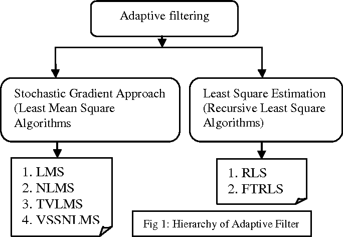
flowchart of adaptive filtering techniques (prototype).

Kalman Filter works on prediction-correction model used for linear and fourth dimension-variant or time-invariant systems. Prediction model involves the actual organization and the process dissonance .The update model involves updating the predicated or the estimated value with the ascertainment racket. Kalman gain is calculated based on RLS algorithm in order to attain the optimal value within less amount of time.

Recursive Least Squares is based on weighted least squares in which previous values taken in account for determining the future value. Each weight is exponentially assigned to each previous value of the bodily system. The weights are updated recursively based on retention.

Notable Differences:

Computational Fourth dimension complexity of RLS

Computational Fourth dimension complication of Kalman Filter

RLS is faster than Kalman Filter.
Accurateness of Kalman Filter is high.
Kalman Filter is based on State-Space model where we need to model entire organization to achieve optimal value.

Kalman filter and Polynomial regression

Polynomial regression is a method of function approximation. Nosotros accept a data set and nosotros have to determine the functional relationship, which is oftentimes expressed by estimating the probability density p(z|10). Under the assumption that this probability is a Gaussian, nosotros become the to the lowest degree squares solution every bit a maximum likelihood estimator.

Since Linear dynamic systems are country space models, we assume that the data we observe is generated by the application of a linear transform. The model we come with is the probability of a time serial. The process and so predicts the next value of a time series.

Polynomial regression does function approximation, Kalman filtering does fourth dimension serial prediction.

The time series prediction is a special case of function approximation. Both the models are modeled from different assumptions on the data they discover.

Conclusion

The Kalman filter is relatively quick and piece of cake to implement and provides an optimal estimate of the condition for ordinarily distributed noisy sensor values under certain conditions. Mr. Kalman was so convinced of his algorithm that he was able to inspire a friendly engineer at NASA. And and so this filter helped for the first time in the Apollo Guidance Estimator at the moon landings .

Useful links:

The Jupyter Notebook Collection of Roger Labbe.
The amazing video series of Michel van Biezen
Kalman Filters in Pictures .
The the blog post of Vivek Yadav .
The amazing mail by David Silver.